How to cope with the variability and complexity of person name variables used as identifiers.
This is the fifth article of our journey into the Python data exploration world. A list of the published articles you can find
here
(and the source code
here
). So let’s start then.
Methods of Name Matching
In statistical data sets retrieved from public sources the names (of a person) are often treated the same as metadata for some other field like an email, phone number, or an ID number. This is the case in our sample sets:
When names are your only unifying data point, correctly matching similar names takes on greater importance, however their variability and complexity make name matching a uniquely challenging task. Nicknames, translation errors, multiple spellings of the same name, and more all can result in missed matches. (
rosette.com)
That’s precisely the situation we are confronted now:
Our twitter data set contains a
Name
variable, which is set by the Twitter user itself. Dependent on the person’s preference it may
-
a complete artificial name
-
surname, last name (or vice versa)
-
only last name
-
abbreviation sure name, abbreviation middle name, last name
-
his full name, but did some misspelling by accident
-
etc. etc. etc.
These leaves us with some data quality and normalization challenges, which we have to address so that we can use the
Name
attribute as a matching identifier.
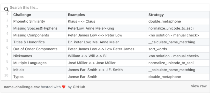
Some of the challenges — as well as our strategy how we want to tackle them — are described in the below table. Each of the method used to address a challenge will be explained in this article and is part of the
Github tutorial source code
.
Let’s start then, by addressing the challenge of
Titles&Honorifics
,
Missing Components,
and some other anomalies first.
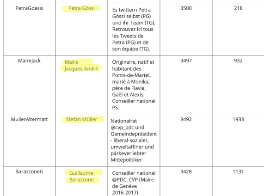
We are in the lucky position that our list is manageable from a number of records point of view, i.e., we can do a manual check about the anomalies and titles used in “Name” attribute.
Name Cleanser Step
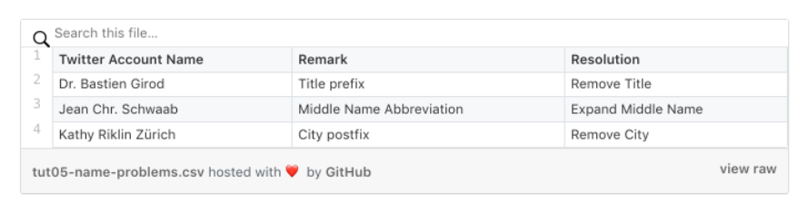
Our quality review shows that the Name field seems to have a good quality (no dummy or nicknames used). However we found some anomalies, as shown below:
We fix these anomalies in our program in a first cleaning step. To stay generic, we use once again our yaml configuration file and add two additional parameters.
-
twitterNameCleaner which consists of a list of keywords which must be removed from any twitter account name
-
twitterNamesExpander which expands each Twitter account name abbreviation substring to a full name string.
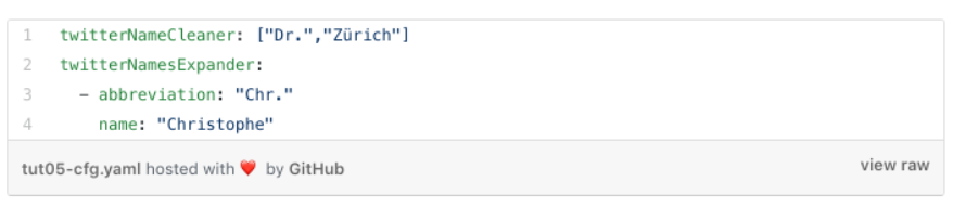
Our country-specific yaml file is enhanced by the following entries.
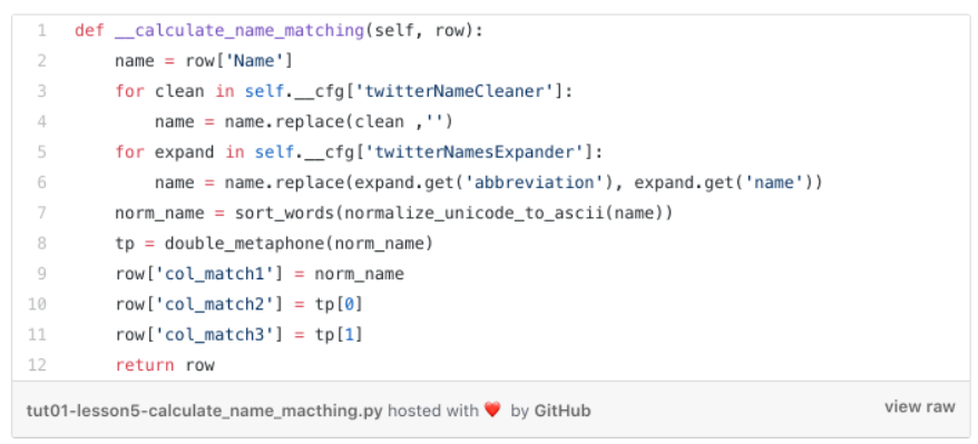
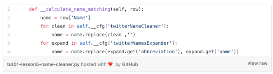
The cleansing step is called in the below method, which assesses every row of our Twitter table (its integration into the program is explained later)
Pretty straightforward by using the String
replace method
-
we remove every keyword found in the
twitterNameCleaner list from the
Name attribute (replace it with ‘’)
-
we replace every abbreviation found in the
twitterNamesExpander dictionary through its full name.
For our next normalizing step, we introduce an approach which has its origin in the time when America was confronted with a huge wave of immigrants 100 years ago.
Double Metaphone Algorithm
The principle of the algorithm goes back to the last century, actually to the year 1918 (when the first computer was years away).
Just as side information (should you ever participate in a millionaire quiz show), the first computer was 23 years away
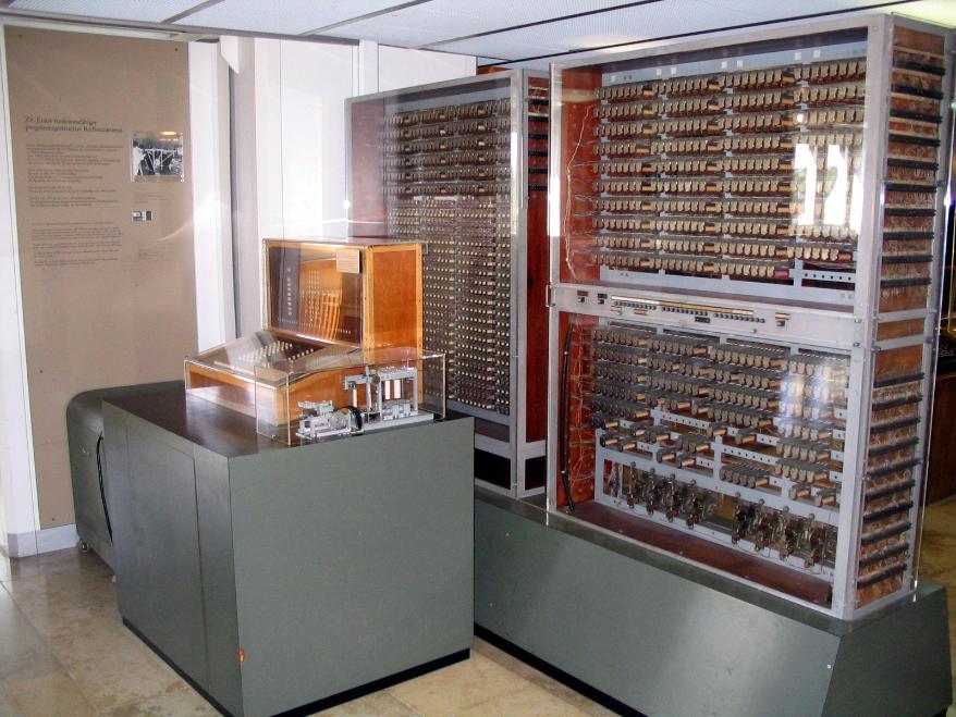
The Z3 was a German electromechanical computer designed by Konrad Zuse. It was the world’s first working programmable, fully automatic digital computer. The Z3 was built with 2,600 relays, implementing a 22-bit word length that operated at a clock frequency of about 4–5 Hz. Program code was stored on punched film. Initial values were entered manually (
Wikipedia
)
A Z3 replica at the Deutsche Museum (
CC BY-SA 3.0)
So back to 1918, in that year Robert C. Russell of the US Census Bureau invented the Soundex algorithm which is capable of indexing the English language in a way that multiple spellings of the same name could be found with only a cursory glance.
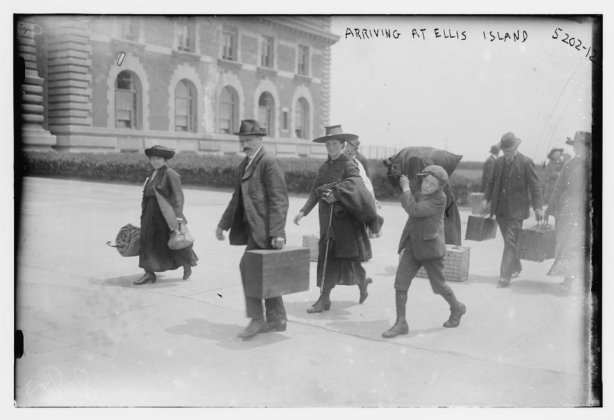
Immigrants to the United States had a native language that was not based on Roman characters. To write their names, the names of their relatives, or the cities they arrived from, the immigrants had to make their best guess of how to express their symbolic language in English. The United States government realized the need to be able to categorize the names of private citizens in a manner that allowed for multiple spellings of the same name (e.g. Smith and Smythe) to be grouped. (read the full story
here
)
Immigrants arriving at Ellis Island — Wikipedia —
Commons Licence
The Soundex algorithm is based on a phonetical categorization of letters of the alphabet. In his patent, Russell describes the strategy assigning a numeric value to each category. For example, Johnson was mapped to J525, Miller to M460 etc.
The Soundex algorithm evolved over time in the context of efficiency and accuracy and was replaced with other algorithms.
For the most part, they have all been replaced by the powerful indexing system called
Double Metaphone
. The algorithm is available as open source and its last version was released around 2009.
Luckily there is a Python library
available
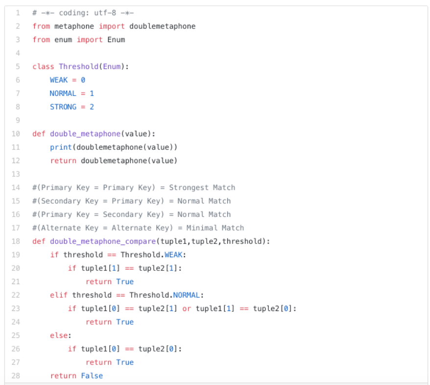
, which we use in our program. We write some small wrapper methods around the algorithm and implement a compare method.
The
doublemetaphone
method returns a tuple of two characters key, which are a phonetic translation of the passed in word. Our
compare
method shows the ranking capability of the algorithm which is quite limited.
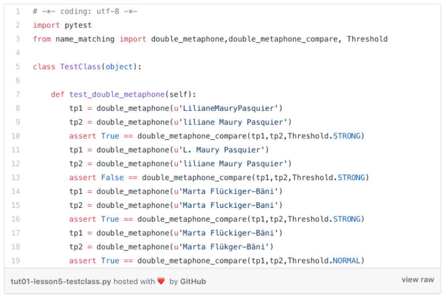
Let’s run some verification checks to assess the efficiency of the algorithm by introducing the
test_class.py
which is based on the Python
pytest
framework.
The pytest framework makes it easy to write small tests, yet scales to support complex functional testing for applications and libraries. (
Link)
Its usage is straightforward and, you can see the test class implementation below
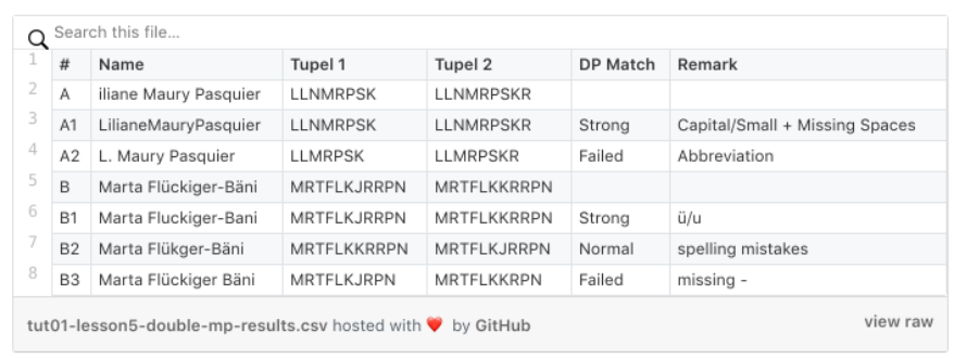
The tests result are shown below. We used two names (A+B) and were checking with some changed names (A1/A2+B1/B2/B3) the efficiency of the algorithm.
-
A1+B1 passed the Strong match check. So missing spaces and ü/ä replacements with u/a seems not affecting the double metaphone key generation
-
B2 passes the Normal match. Spelling mistakes are covered by the algorithm as well
-
A2 + B3 are failing. A2 uses an abbreviation of a name part, which cannot be coped with. This behavior we had to expect and decided to introduce the name expander algorithm (see above). B3 failed due to missing “-”. This was unexpected, but we cover this behavior with a second name cleanser step.
Name Cleanser Step 2
Our small test run has shown that the following additional cleaning steps are beneficial:
-
We have to get rid of any special character which could result in a failure
-
Out of order components, i.e., the last name before the first name affects the phonetic key generation. Therefore best is to sort the name components alphabetically to increase matching accuracy.
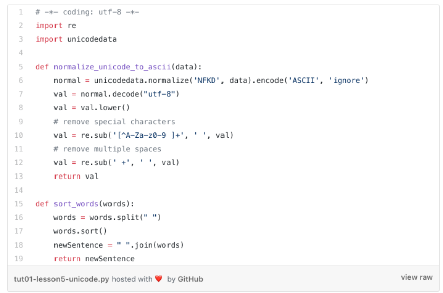
Besides getting rid of any special character, we decide to remove any Unicode character, i.e. in Switzerland, multiple German (ä,ö,ü), French (à,é,è) or Italian umlaut are used, and we want to get rid of them as well.
The below
normalize_unicode_to_ascii
method uses the
unicodedata
library to convert the name to ASCII and then change all character to lower case. Afterward, two regular expressions are used to remove the special characters, as well as multiple spaces.
Regular expression operations are a powerful mechanism but not easy to understand for a novice. You may work through the
following tutorial
to get the first impression of this powerful approach.
-
Just one explanation, the regular expression term
‘[^A-Za-z0–9 ]+’ means take any number of characters between ‘A-Z’ + ‘a-z’ + ‘0–9’ +‘ ‘ out of the passed in string. ^[]+ are special characters in the regular expression. The expression sequence can be translated to “strip the string from any special character.”
-
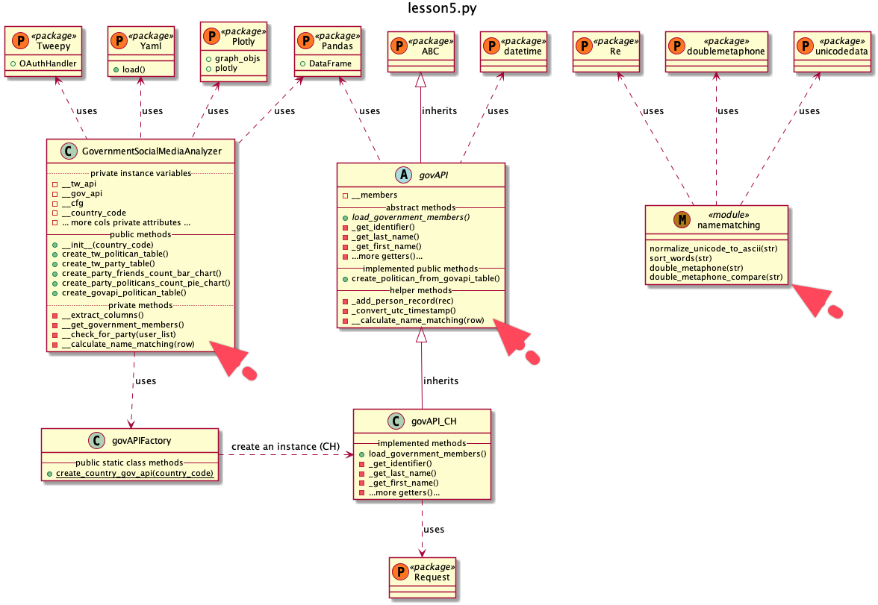
The Beauty of the Data Frame “Apply” Method Establish the calculate_name_matching method in both classes
We have now all our name cleanser, normalization, and phonetic key generator methods together (bundled in the
namemachting.py
module) and can finally construct our name matching identifiers creation method(s)
calculate_name_matching
for our two classes
govAPI
and
GovernmentSocialMediaAnalyzer.
One new module and two new methods are added
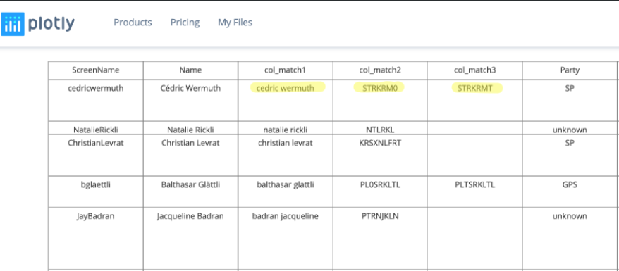
Both of the classes get a new method, which we apply to their Panda data frames and each method creates three new identifier attributes (
col_match1, col_match2, col_match3
). The three columns can then be used to merge the two data frames.
The method for our
governmentAPI
class looks as follows:
So for our
govAPI
class as follows. It’s an implemented method in our abstract class. The method is used for any implemented sub-class (refer to the factory design explained in our
earlier tutorial
)
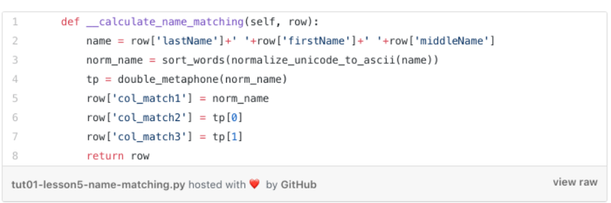
The implementation is straightforward, we normalize the person’s name of each table (from the government API we got back three independent attributes, from the Twitter API one account name) and then calculate the two double metaphone identifier strings. All three new values we append to the passed in row.
Don’t call us we call you: “The Hollywood Principle”
One question is still open: “How do we use our new methods to get the data frame enhanced by the three columns with its calculated values for each row?
apply() can apply a function along any axis of the dataframe
This is a nice and elegant way to do any calculation on each row or column of a data frame.
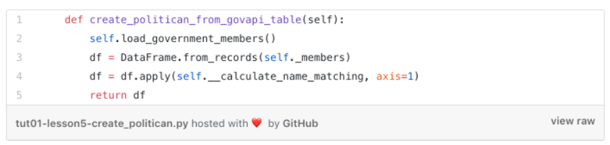
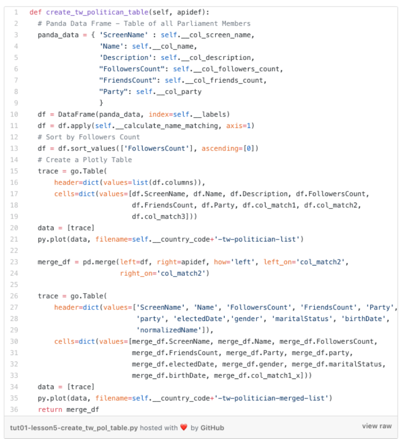
Below you see the enhanced
create_politican_from_govapi_table
method. On code line 4 we newly call the
apply
method of the data frame (
df
) and pass in as a parameter our method name
self.__calculate_name_matching
and instruct the
apply
method to call our method for each row (
axis=1
).
Now the Panda data frame
-
iterates through each data row, which represents a data record of a dedicated politician
-
calls our
self.__calculate_name_matching method
-
passes in the data row as a parameter and stores back the data row returned by the method call (which three new columns).
Very nifty isn’t it? We didn’t have to code any kind of loops which are fetching data, checking for the end of loop conditions and so on. We just have implemented the method which can be passed to the
apply
method.
This kind of interaction is a well-known design principle in IT, known under the name “Hollywood Principle”, which the excellent
blog article of Matthew Mead
describes as follows:
The essence of this principle is “don’t call us, we’ll call you”. As you know, this is a response you might hear after auditioning for a role in a Hollywood movie. And this is the same concept for the software Hollywood Principle too. The intent is to take care to structure and implement your dependencies wisely.
Think about our implementation above. Our
calculate_name_matching
method is completely decoupled of the panda data frame implementation. Our method gets just a row dictionary as an input, which we can manipulate and can give back at the end as the return value. We are completely unaware that there is a massive panda data frame implementation involved and don’t have any dependency on it.
At its most basic level, the principle is about reducing the coupling in a software system. It gets back to the well known phrase in software development: loose coupling and high cohesion. You can keep classes loosely
coupled by ensuring that you don’t have unnecessary references and you are referencing classes and other subsystems properly. Although the Hollywood Principle does not dictate anything about cohesion, it is an important aspect too.
Cohesion is about keeping your classes true to their intent and not allowing their behavior to expand beyond its core purpose. Like high coupling, low cohesion doesn’t tend to cause systems to be unstable or not work properly, but will likely lead to difficulty in maintaining the software.
Enough design teaching for today, when we run our program both plotly politician tables are enhanced by 3 new attributes, which allows us to join them together finally (uff… quite some conceptual work we had to do)
Finally, Join the Data Frames
We now have to join the two data frames, which is one of the many combining and merging possibilities which Panda is offering. Refer to the following article by
datacarpentry.org
, which gives a good introduction to the overall topic.
Another way to combine DataFrames is to use columns in each dataset that contain common values (a common unique id). Combining DataFrames using a common field is called “joining”. The columns containing the common values are called “join key(s)”. Joining DataFrames in this way is often useful when one DataFrame is a “lookup table” containing additional data that we want to include in the other.
This is achieved by the
merge
method which can be applied to a Panda data frame (see code line 23 below). You have to provide as parameters
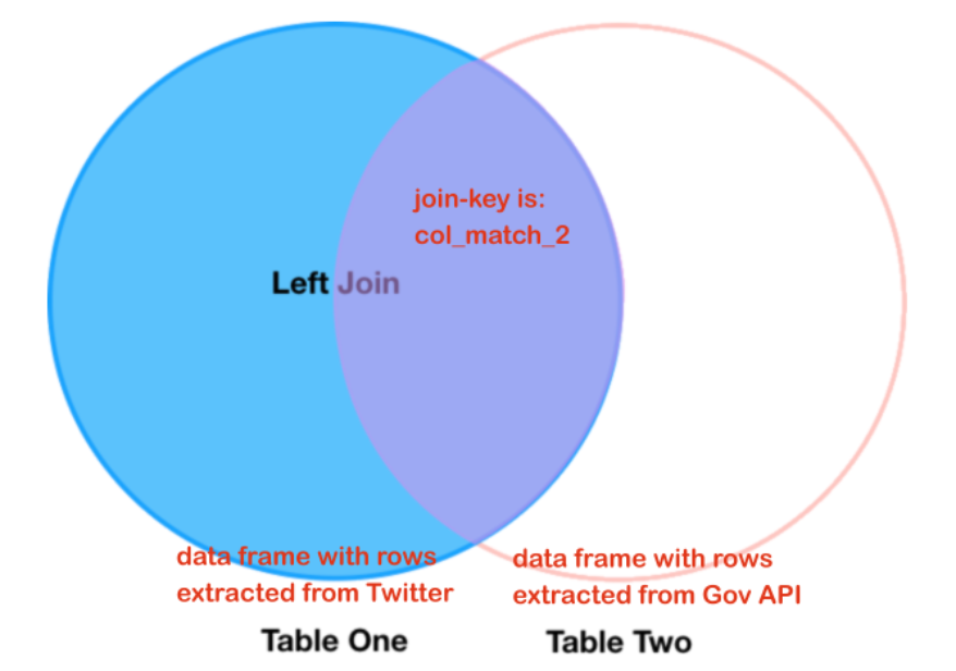
We indicate an “outer left” join (
how=left)
which can be visualized as follows
Omitting the
how
parameter would result in an inner join
“Inner Join” means only take over rows which are matching, “Left Join” means to take over ALL row of the left data frame. If there is no matching right table record, fill the relevant record with “NaN” values.
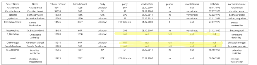
Our new Plotly table
CH-tw-politican-merged-list
has such kind of entries.
Well, that means our matching strategy still misses entries. Let’s compare the Pie Chart of our merged table, with the initial one:
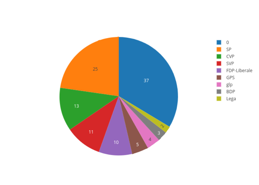
Twitter User per Party (merged with gov API source)
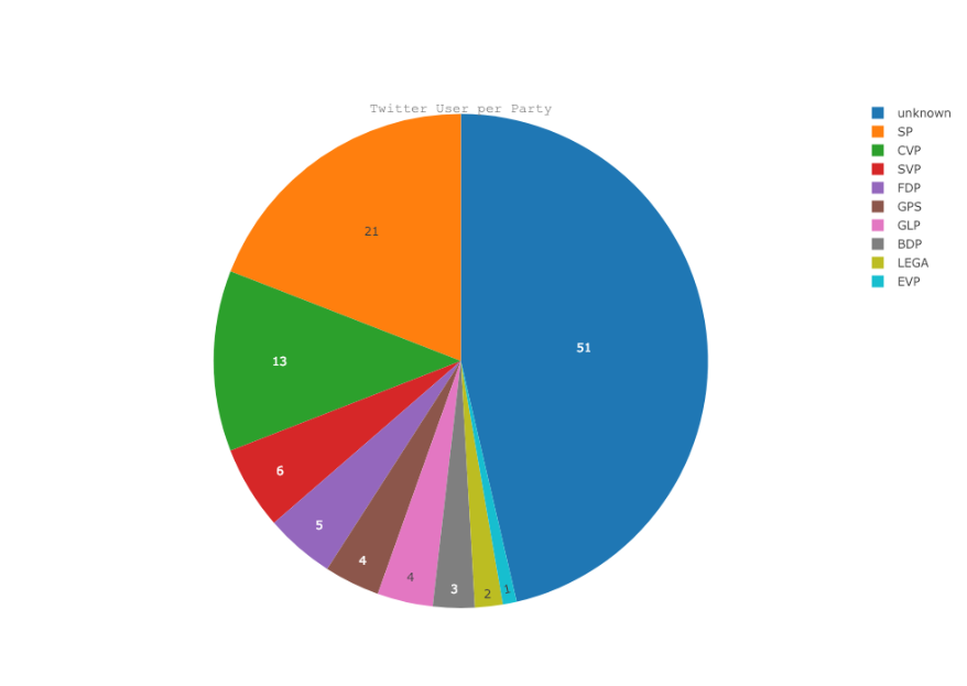
The initial one (refer to this
article
) missed 51 one, with our simple merge strategy we could identify another 14 entries.
Twitter User per Party (just using Twitter API information)
So, we are not there yet (argh…), but enough for today, in the next session we try to adapt our matching strategy so that we can reduce the unknown once again.
The source code you can find in the corresponding
Github project
, a list of all other articles
here
.